12  Volume and Subsurface Scattering Processes

\[ \def\oi{{\omega_i}} \def\os{{\omega_s}} \def\Oi{{\Omega_i}} \def\Os{{\Omega_s}} \def\d{{\text{d}}} \def\D{{\Delta}} \def\do{{\d\omega}} \def\Do{{\Delta\omega}} \def\doi{{\d\omega_i}} \def\dos{{\d\omega_s}} \def\Doi{{\D\omega_i}} \def\Dos{{\D\omega_s}} \def\H{{\mathbf{H}}} \newcommand{\cM}{\mathcal{M}} \newcommand{\cL}{\mathcal{L}} \]

Now we turn our attention to subsurface scattering and volume scattering. While superficially different, they involve the same forms of light-matter interaction and are modeled in the same way. This chapter is concerned with local events — absorbing (Section 12.1) and scattering (Section 12.2) photons by particles at a particular point in a medium. Understanding the local behaviors will then allow us to build a general framework in the next chapter to reason about subsurface and volume scattering globally.

12.1 Absorption

We start by modeling absorption in this chapter, and the way we build the models is fundamental to how scattering will be dealt with later.

12.1.1 A Simple Case: Collimated Illumination on Uniform Medium

Imagine that a beam of light hits a volume of particles. The light is collimated in that all photons travel along the same direction. We take a slice of the material perpendicular to the incident direction. The slice is so thin that no particles in that material cover each other from the direction of the incident light. This is shown in Figure 12.1 (a). We also, for now, assume that the medium is uniform in that the number concentration \(c\) (i.e., the number of particles per unit volume) of each slice is exactly the same.

Figure 12.1: Conceptual model to help reason about photon absorption. (a): the setting for calculating the radiance reduction over a very thin slice. (b): the radiance reduction over a finite length is calculated by accumulating the radiance reduction over infinitely many thin slices.

Say the slice has a depth of \(\D s\) and a geometrical cross-sectional area of \(E\). All the particles have the same geometrical cross-sectional area of \(\epsilon_g\). In the simplest model, a photon is absorbed whenever it hits a particle. In reality, the chance of absorption can be higher or lower. The effective area available for absorption is:

\[ \epsilon = \epsilon_g Q_a, \]

where \(Q_a\) is called the absorption efficiency and is usually smaller than 1 for molecules (which have small \(\epsilon_g\)) and greater than 1 for large particles (whose \(\epsilon_g\) can be large). \(Q_a\) is wavelength dependent, so we should have written it as \(Q_a(\lambda)\), but we will omit the wavelength in our notations for simplicity’s sake. In physics, \(\epsilon\) is called the absorption cross section of the particle; it characterizes the intrinsic capability of a particle to absorb photons. Mind the subtle but important difference between the geometrical cross-sectional area and the cross section of a particle.

The question we are interested in is, if the incident radiance is \(L\), what is the radiance leaving the slice \(L+\D L\)? By convention, \(\D L\) is defined as the exitant radiance minus the incident radiance and, in this case, has to be negative. The percentage of photons that are absorbed by this slice of particles (\(-\frac{\D L}{L}\)) is equivalent to the cross-sectional area of the slice that is covered by the total cross sections of the particles:

\[ -\frac{\D L}{L} = \frac{cE\D s\epsilon}{E}, \tag{12.1}\]

where \(c\) is the particle concentration of the slice, and \(E\D s\) is the total volume of the slice. So \(cE\D s\) is the number of particles in this thin slice, and \(cE\D s\epsilon\) is the total cross section of all the particles. Given the assumption that no particles are covering each other, \(\frac{cE\D l\epsilon}{E}\) is then the percentage of the thin slice’s cross-sectional area that is available for photon absorption and, thus, the percentage of the incident photons that are absorbed. The negative sign on the left-hand side of Equation 12.1 signals the fact that \(\D L\) is negative.

We rewrite Equation 12.1 as Equation 12.2: \[ \frac{\D L}{\D s} = -c\epsilon L = -\sigma_a L, \tag{12.2}\]

which shows that the amount of photon absorption per unit length (\(\frac{\D L}{\D s}\)) is proportional to the current amount of photons up to a scaling factor \(c\epsilon\). In the computer graphics literature, \(c\epsilon\) is called the absorption coefficient, denoted \(\sigma_a\).

Bouguer-Beer-Lambert’s Law

When \(\D s\) approaches infinity, we can rewrite Equation 12.2 as a differential equation:

\[ \frac{\d L}{\d s} = \lim_{\D s \rightarrow 0}\frac{\D L}{\D s} = -\sigma_a L \tag{12.3}\]

This equation is a classic case of exponential decay, and its solution is given by:

\[ L(s) = L_0 e^{-\sigma_a s}. \tag{12.4}\]

where \(L_0 = L(0)\) is the initial radiance of the light before interacting with the particles, as visualized in Figure 12.1 (b), \(L(s)\) denotes the radiance at a particular length \(s\).

Equation 12.4 allows us to calculate the remaining radiance after the light travels a length \(s\). Equation 12.4 is called the Bouguer-Beer-Lambert’s law (BBL), which is a geometrical optics’ simplification of the electromagnetic theory of light-matter interaction where the matter is purely absorptive (Mayerhöfer, Pahlow, and Popp 2020).

An Alternative Derivation

An equivalent way of deriving the BBL law is the following. We divide the entire volume (with a total length of \(s\)) into \(N\) thin slices, each with a length of \(\D s\). After the first slice, the surviving portion of the initial radiance is \(L = L_0(1-\sigma_a \D s)\), so after going through all the \(N\) slices, the remaining radiance is given by:

\[ L_N = L_0(1-\sigma_a \D s)^N = L_0(1-\sigma_a \frac{s}{N})^N. \tag{12.5}\]

Now when \(\D s\) becomes infinitesimally small, \(N\) approaches infinity, so the limit of the remaining radiance as a function of the total length \(s\) is given in Equation 12.6, which is the same as Equation 12.4.

\[ L(s) = \lim_{N \rightarrow \infty}L_0(1-\sigma_a \frac{s}{N})^N = L_0 e^{-\sigma_a s}. \tag{12.6}\]

12.1.2 Absorption Coefficient

The absorption coefficient is an important measure of the medium’s ability to absorb photons. It has a unit of \(\text{m}^\text{-1}\), which means it is not bound by 0 and 1. One way to interpret the absorption coefficient is to observe that \(\sigma_a \d s = \d L/L\), which is the fraction of the radiance absorbed or the probability of light absorption by an infinitesimal slice. So \(\sigma_a = (\d L/L)/\d s\) can be interpreted as the probability density of photon absorption, i.e., the probability of absorption per unit length traveled:

\[ \sigma_a = \lim_{\D s \rightarrow 0} \frac{\D L}{L}/\D s = \frac{\d L}{L \d s}. \]

Like any density measure, absorption coefficient is most useful when it is integrated: when we integrate \(\sigma_a\) over the length that light travels, we get the fraction/percentage of the light absorbed. One can also show that \(1/\sigma_a\) is the expected value of the distance a photon can travel before being absorbed (Bohren and Clothiaux 2006, chap. 5.1.3); this quantity is given the name mean free path (l). To derive \(l\), observe that the probability that a photon is absorbed after traveling a distance \(s\) is \(1-e^{-\sigma_as}\). So the probability density of absorption as a function of the distance \(s\) is:

\[ f(s) = \frac{\text{d}(1-e^{-\sigma_a s})}{\text{d}s} = \sigma_ae^{-\sigma_a s}. \]

So the expected value of \(s\), which we can interpret as the distance a photon can travel on average before being absorbed, is:

\[ l = \int_0^\infty sf(s)\text{d}s = 1/\sigma_a. \tag{12.7}\]

12.1.3 A Few Important Quantities

We can now define a few other commonly used quantities (omitting the wavelength dependence for simplicity). The transmittance \(T\) of a volume with a total thickness of \(s\) is defined as the percentage of the transmitted/unabsorbed photons after traveling the length of \(s\) (Equation 12.8): \[ T = \frac{L(s)}{L_0} = e^{-\sigma_a s}. \tag{12.8}\]

The absorbance \(A\) is the product of \(\sigma_a s\): \[ A = -\ln T = \ln\frac{L(s)}{L_0} = \sigma_a s. \tag{12.9}\]

The absorptance \(a\) of a volume is defined as the percentage of the absorbed photons by the volume, which relates to \(T\) and \(A\) by Equation 12.9: \[ a = 1 - T = 1 - e^{-A}. \tag{12.10}\]

We have seen these definitions in Section 3.2.1. One very nice thing about the absorbance \(A\) is that it is approximately equivalent to absorptance \(a\) when \(A\) is small (which would be true when, e.g., the length \(s\) is very small, as is the case when discussing how a photoreceptor absorbs photons when illuminated transversely).

Another nice thing about absorbance is that absorbances add, because absorption coefficients add. Imagine you have \(n\) kinds of particles mixed up in a medium, each with a different absorption coefficient \(\sigma_a^i\). The overall absorbance of the medium is the sum of the individual absorbance \(A^i\) derived as if the medium is made up of only one kind of particles. That is: \[ A = \sum_i^n A^i = s\sum_i^n\sigma_a^i = s\sum_i^n c^i\epsilon^i, \tag{12.11}\]

where \(c^i\) and \(\epsilon^i\) are the concentration and absorption cross section of the \(i^{th}\) particles. Specifically, \(c^i\) is defined as: \[ c^i = \frac{n_i}{V}, \]

where \(n_i\) is the number of the \(i^{th}\) kind of particles in the material, and \(V\) is the material volume.

This is not a surprising result. As long as particles in a thin slice of this new heterogeneous medium do not cover each other, we can easily extend Equation 12.1 and the rest of the derivation to consider multiple kinds of particles; eventually Equation 12.11 would be a natural conclusion. We will omit the derivation here for simplicity sake.

Equation 12.11 is a nice conclusion to have, because usually we are dealing with hybrid media. For instance, paint is a mixture of binder particles and pigment particles, and a mist is a mixture of water droplets and air particles. If we do not want to model individual matters, we can use a single absorption coefficient to describe the aggregate behavior of the mixture. That absorption coefficient does have a physical meaning: it is the concentration-weighted sum of the individual absorption coefficients.

There are a bunch of other quantities defined in the literature. The state of the definitions is a bit of a mess, largely because different communities use different definitions.

• In visual neuroscience people sometimes use a quantity called specific absorbance (see, e.g., Bowmaker and Dartnall (1980)), which is the absorbance per unit length \(\frac{A}{s}\). Whenever you see a quantity that starts with the word “specific”, chances are that the quantity is defined per unit length. You can see that specific absorbance is actually just our absorption coefficient.

• In scientific communities, especially chemistry and spectroscopy, people define \(\epsilon\), rather than \(c\epsilon\), to be the absorption coefficient. You can see the appeal of doing that — \(\epsilon\) is a more fundamental measure of a medium’s ability to absorb photons, independent of the particle concentration \(c\) (and certainly independent of the traversal length \(s\)).

• The absorbance defined in Equation 12.9 is technically called the Naperian absorbance, because we take the natural logarithm of \(T\). Sometimes people also use the decadic absorbance, which is defined as \(-\log T\). This quantity is also called the optical density.

• Finally, the number concentration \(c\) here is defined in terms of the absolute quantity per unit volume, but sometimes people want to define \(c\) as the molar concentration, which is the number of moles per unit volume. If so, all other derived quantities are then prefixed with “molar”. Next time when you see something like the molar decadic absorption coefficient, you know what it is!

The annoying thing is that people do not always tell you which definition they use. The plea I have to you is to be specific about which definition you use in your writing and tell me when I am being vague!

12.1.4 General Case

So far we have assumed that the absorption coefficient \(\sigma_a = c\epsilon\) is a constant regardless of the position \(p\) in the medium and along any direction \(\omega\). The former property assumes that the medium is uniform, and the latter property is called isotropic¹ in that the medium’s ability to absorb photons is independent of the light direction.

Both assumptions are problematic in practice. The concentration can change spatially and should be denoted \(c(p)\), where \(p\) is an arbitrary position in space. \(\epsilon\) can also change with \(p\) and, more importantly, change with the direction of light incidence \(\omega\). For instance, the particles might not be spherical, so their geometrical cross-sectional area and, thus, the cross section \(\epsilon\) available for absorbing photons can depend on \(\omega\). As a result, the absorption coefficient should generally be denoted \(\sigma_a(p, \omega)\).

Figure 12.2: A conceptual model to help reason about photon absorption in the general case, where the absorption coefficient can vary spatially and directionally. The medium is divided into many tiny elemental volumes, each of which is so small that particles do not cover each from any direction.

Effectively, our conceptual model, shown in Figure 12.2, has to be changed to one where the entire body of particles is divided into many equally-sized volumes (with a length \(\D s\) and an area \(\D A\)), each of which is so small that particles do not cover each other from any direction. The radiance reduction per unit length in a small volume is then expressed as:

\[ \frac{\D L(p, \omega)}{\D s} = -\sigma_a(p, \omega)L. \tag{12.12}\]

Given this model, we can calculate the exitant radiance after light travels a length \(s\) through the medium:

\[ L(p+s\omega, \omega) = L(p, \omega) e^{-\int_0^s \sigma_a(p+t\omega, \omega) \d t}, \tag{12.13}\]

where \(\omega\) is the (unit) direction of the incident radiance, \(L(p, \omega)\) is the incident radiance, and \(L(p+s\omega, \omega)\) is the exitance radiance (radiance toward \(\omega\) leaving the entire medium after traveling \(s\)).

You would notice that for a beam with an oblique incident direction, the distance traveled, say \(\D s'\), can be different (longer or shorter than) from \(\D s\). Our model can account for this by folding the factor \(\D s'/\D s\) specific to a particular direction \(\omega'\) into the absorption coefficient \(\sigma_a(p, \omega')\). Note that the \(\D s'/\D s\) factor should be the average for all the incident photons with the same direction \(\omega'\) across the entire \(\D A\).

12.1.5 Nature and Applicability of the Model

The absorption model (the BBL law) derived before (Equation 12.4 and Equation 12.13) is a continuous one, but it is derived based on modeling discrete particles and events. It is another example of the modeling methodology discussed on Section 11.2.1.

Equation 12.13 seems to suggest that absorption coefficient \(\sigma_a(p, \omega)\) is continuously defined at any position \(p\) in the medium along any direction \(\omega\). It is not true. For starters, concentration \(c\) is not continuous. Rather, it exhibits the triphasic profile shown in Figure 11.2. As we keep shrinking the size of the volume to the molecular scale, eventually the concentration depends on whether the tiny volume contains any molecules or not, so it becomes wildly discontinuous, not to mention the headache of dealing with a partial molecule in a volume — should it be counted or not? In general, the absorption coefficient can be an arbitrary discontinuous function that is not integrable.

What about Equation 12.4 where the absorption coefficient is uniform so we do not have to take the integral? Well, that is a lie too: concentration is not continuous, so it cannot be uniform everywhere, and, by extension, the absorption coefficient cannot be a constant everywhere either. So Equation 12.3 is technically wrong when we let \(\D s \rightarrow 0\) (i.e., \(N \rightarrow \infty\)), which is necessary for us to construct the differential equation (or take the limit in Equation 12.6). For Equation 12.3 to be true, the concentration/absorption coefficient must be a constant everywhere, which can be true only if the volume is continuous.

What has to happen is that the limit of \(\D s\) cannot be literally 0 and the limit of \(N\) cannot be infinity. What we do is to keep reducing \(\D s\) to the point where the concentration (and thus absorption coefficient) is insensitive to slight perturbation of \(\D s\) (i.e., operating in the stable range in Figure 11.2), and call it the concentration/absorption coefficient of that specific \(\D s\). And we repeat this for all the \(\D s\). This certainly applies to the general-case models in Equation 12.12 and Equation 12.13, where we iterate over not the thin slices \(\D s\) but all the tiny volumes (\(\D A \times \D s\)). So all the integral symbols are secretly summing over an extremely fine-grained grid.

How big of an error are we introducing here? Technically, we should sum all \(N\) slices across the total traversal length \(s\) in Equation 12.5. If we assume \(\D s\) to be very small (even though not infinitesimal) compared to \(s\), \(N\) would be large, so taking the integration (equivalent to letting \(N \rightarrow \infty\)) would be very close to summing over \(N\). Similarly, the integral in Equation 12.13 should have been a summation of the concentration in each of the \(N\) slices. If you want to be pedantic, however, the integration there is exact: we can model \(c\) as a piece-wise function, where the value at each piece is the concentration of the corresponding volume. Integrating over a piece-wise function is the same as summing all the pieces. Only the exponential expression in Equation 12.13 is inexact.

The discontinuity of the medium is, of course, orthogonal to the discontinuity and non-uniformity in the light field itself. For instance, the fact that we use \(\frac{cE\D l\epsilon}{E}\) as the percentage of photon absorption in Equation 12.1 (and implicitly in Equation 12.4) assumes that the irradiance of the incident illumination is continuous and uniform in the small volume. This is technically not true because photons are discrete packets of energy. But in practice this is not a concern because we can assume that there is an enormous amount of photons incident on the small volume, and these photons are randomly distributed.

In essence, we are using the aggregated behavior of many photons to model the behavior of a small volume. This is similar to the microfacet models, where we use the aggregated behavior of many microfacets to statistically model the behavior of a small macro-surface.

This sort of modeling strategy is a weird case where the discrete model provides the “ground truth”, which is approximated by a continuous model. I say ground truth — to the extent that the geometrical optics can approximate the electromagnetic theory of light-matter interaction. The BBL law fails when the wave nature of photons has to be considered (Mayerhöfer, Pahlow, and Popp 2020).

12.2 Scattering

Scattering is much more difficult to reason about than absorption, primarily because a scattered photon is not “dead” and continues to participate in light-matter interaction. The way to study scattering is to first understand the behavior of a single scattering event and then consider the overall behavior of a large of collection of particles.

This section focuses a single scattering event (Section 12.2.2), and the next section discusses the general case where a large collection of particles interacts with photons. Before all these, though, it is useful to first build some intuitions as to why there is a distinction between a single scattering event and scattering by a particle collection and explicitly lay out the assumptions made for the rest of our discussions (Section 12.2.1).

12.2.1 Scattering by a Particle vs. a Collection of Particles

In geometric optics terms, scattering can be thought of as an event that takes place between a photon and a particle. In the real world, however, objects and media are usually made of a large collection of particles, which introduces two complications: multiple scattering and interference.

Multiple Scattering

First, it is possible that a scattered photon, after traveling a certain distance, meets another particle and gets scattered again. This makes it considerably more difficult to analyze the effect of scattering by a medium than does the scattering of a single particle.

Figure 12.3: Left: The atmospheric scattering of the sand coming from the Sahara during Harmattan glows in the sun and gives a hazy view of the remote mountains. Nigeria’s National Mosque is in the foreground; from Kipp Jones (2005). Right: illustrations of the glow of the sun and the haze. Both are due to scattering, and the difference is purely visual but not fundamental.

Look at Figure 12.3 (left) taken during Harmattan, where the atmosphere is full of sand and dust blown from the Sahara. The large collection of particles in the atmosphere scatters light, glowing the sun and giving the remote mountains a hazy view. The right panel illustrates the scattering events that give rise to the glow and the haze.

Without scattering, sunlight enters the eye directly. With scattering, some photons from the sun are first knocked out of the view and could potentially be then scattered again back to the eye. Some photons that enter the eye might even come from nearby objects other than the sun. The scattering creates a glow around the sun, and, for the observer, the sun appears larger than it actually is. The hazy view of the mountains is created by exactly the same scattering processes. The photons that enter the eyes are mixed up from different parts of the mountains and from other objects. The mountains appear hazy rather than glowing as the sun does simply because the sun has a higher brightness contrast against the background than does a region on the mountain. So the distinction between “glow” and “haze” is nothing more than a visual difference at a superficial level rather than anything deeper in physics.

You can see why multiple scattering by large collections of particles poses challenges to our analysis. If a photon is scattered once in the medium, the only effect of scattering would be to knock photons out of our line of sight, and thus, remote objects would only look dimmer rather than hazy. In this case, scattering would function exactly like absorption, for modeling purposes at least. With multiple scattering, we have to track not only photons that are scattered out but also photons that are scattered into the rays that enter our eyes². This is a daunting task considering that we are usually dealing with millions of particles and billions of photons, if not more.

If one were to be absolutely pedantic, we can distinguish the following cases:

1. a single scattering event, where a photon meets a particle and is scattered away;
2. single scattering, where a photon is scattered once by a medium (a large collection of photons), which is under
   1. a collimated illumination, so the radiance of a ray can only be weakened because photons are scattered to other directions,
   2. an arbitrary illumination, so the radiance of a ray can be both weakened and augmented (by photons scattered from other directions);
3. multiple scattering, where a photon is scattered multiple times by a medium, so the radiance of a ray can both be weakened and augmented.

Section 12.2.2 studies Case 1 and Case 2(a) together, because the latter is the statistical consequence of the former. Chapter 13 studies Case 2(b) and Case 3 together because they have the same observable effects and, thus, are modeled in the same way.

Interference and Coherence

Second, when there is a large collection of particles, the scattered radiation fields of individual particles can interfere with each other. The exact impact of interference can only be calculated by considering the wave nature of the light. But to the first order, the inference depends on how densely packed the particles are.

In fact, the specular surface scattering we discussed in Section 11.1 is just a macroscopic approximation of the microscopic volume scattering where particles interfere non-randomly. In a mirror or a glass of water, the particles/molecules are very densely packed to the point that the distance between two particles is smaller than the wavelength of the light. As a result, the scattering is coherent, which gives rise to the illusion of a specular surface. One can show that the Fresnel equations are the solution to the Maxwell’s equations when surface particles are densely packed.

Why would the particle density matter? If particles are very close to each other, their radiation fields are close too, so the interference is stronger and cannot be ignored. More importantly, when particles are close to each other, their spatial positions can no longer be treated as random, so the interference can become coherent. Imagine you drop particles into a vast empty space; the particle sizes are much smaller relative to the space, so their spatial distribution can be roughly described as random. But if the particles are very densely packed, where the next particle can be is very much restrained, so their positions are highly correlated, leading to coherent scattering.

We will generally assume incoherent scattering unless otherwise noted, where individual scattering events interfere each other in random ways, so we are spared of the complication of thinking of the wave nature of the photons. Under this assumption, the total power scattered by a collection of particles is the same as the sum of the power scattered by the individual particles. This happens when the particles are sufficient sufficiently distant (separated by more than multiple wavelengths) and their spatial arrangements are uncorrelated.

12.2.2 A Single Scattering Event

Scattering Efficiency and Coefficient

Intuitively, scattering has a similar effect as absorption: it weakens the radiance by taking photons away from a beam of light. The difference is that scattered photons are not dead; they are re-directed to other directions. We can define two important quantities, one to characterize a particle’s ability to scatter photons and the other to characterize a medium’s ability to scatter photons.

Similar to the situation in absorption, the intrinsic capability of a particle to scatter photons is defined by the particle’s scattering cross section \(\epsilon_s\), which itself is the product of the geometrical cross-sectional area of the particle \(\epsilon_g\) and the scattering efficiency \(Q_s\). We can then define the scattering coefficient \(\sigma_s\) of a medium (a large collection of particles), which characterizes the ability of the medium to scatter photons away from its incident radiance. \(\sigma_s\) is the product of the particle concentration of the medium \(c\) and the particle’s scattering cross section \(\epsilon_s\). Again, \(\sigma_s\) has a unit \(\text{m}^\text{-1}\) and is not bound by 0 and 1; it is best interpreted as the probability density (i.e., probability per unit length) of light being scattered away. Of course, both the scattering efficiency and scattering coefficient can vary spatially, angularly, and spectrally.

The effects of scattering and absorption add up, because they both weaken a radiance. We can extend Equation 12.13 to consider scattering (again omitting the wavelength from the equations):

\[ L(p+s\omega, \omega) = L(p, \omega) e^{-\int_0^s (\sigma_a(p+t\omega, \omega) + \sigma_s(p+t\omega, \omega)) \d t}, \tag{12.14}\]

where \(\sigma_s(p, \omega)\) is the scattering coefficient at \(p\) toward the direction \(\omega\).

Rearranging the terms, we can express the transmittance between \(p\) and \(p+s\omega\) along the direction \(\omega\), denoted \(T(p \rightarrow p+s\omega)\): \[ T(p \rightarrow p+s\omega) = \frac{L(p+s\omega, \omega)}{L(p, \omega)} = e^{-\int_0^s (\sigma_a(p+t\omega, \omega) + \sigma_s(p+t\omega, \omega)) \d t}. \tag{12.15}\]

Equation 12.14 can be derived using the same idea as that used for deriving the absorption equation in Section 12.1.1 by modeling a thin layer \(\D x\) — with an additional assumption that \(\D x\) is so thin that a photon is scattered at most once before leaving \(\D x\). Therefore, scattering by a single particle has the same effect as absorption: they both take the photon out of the radiance, and that is why the absorption equation (Equation 12.13) can be directly extended here.

Think of the applicability of Equation 12.14: it says that the radiance of a ray can only be weakened. If the incident light has only one direction (e.g., a collimated beam), Equation 12.14 is true when a photon is scattered at most once in the medium. This is because a scattered photon will not have a chance to get back to the ray. If the incident light is not mono-directional, e.g., diffuse illumination, Equation 12.14 in general does not apply — even if we consider only single scattering. This is because photons originally not along the direction \(\omega\) can be scattered toward it through just one single scattering event. We can see how limited Equation 12.14 is: it applies only when the illumination is collimated and we assume only single scattering. We will relax this constraint later.

Just like the absorption case (Equation 12.11), if a medium is mixed with different particles, each with a different scattering coefficient, the overall scattering coefficient is the sum of the individual scattering coefficients as if the medium is made up of a particular kind of particles.

The sum of the scattering coefficient and absorption coefficient is called the extinction coefficient or attenuation coefficient, denoted \(\sigma_t(p, \omega)\):

\[ \sigma_t(p, \omega) = \sigma_a(p, \omega) + \sigma_s(p, \omega). \]

The ratio between the scattering coefficient and the attenuation coefficient is called the single-scattering albedo of the medium:

\[ \rho = \frac{\sigma_s(p, \omega)}{\sigma_t(p, \omega)}. \]

This albedo can be seen as the volumetric counterpart of the surface albedo discussed in Equation 10.11. The two forms of albedo have the same physical meaning: the fraction of the incident energy that is scattered away (i.e., not absorbed). A dark medium (e.g., smoke) has a lower albedo, and a bright medium (e.g., mist) has a higher albedo.

The sum of the scattering and absorption cross sections is called the extinction cross section or attenuation cross section, denoted \(\epsilon_t = \epsilon_a + \epsilon_s\). And of course \(1/\sigma_t\) is the mean free path in a medium where both absorption and scattering take place, i.e., the mean distance a photon can travel without being absorbed or scattered away.

12.2.3 Scattering Direction Distribution: Phase Function

While the scattering efficiency (coefficient) characterizes how well a particle (medium) is able to scatter photons, it tells us nothing about the direction of scattering. The direction of a single scattering event is characterized by the phase function \(f_p(p, \os, \oi)\), which can be interpreted as the probability density function that a photon incident from a direction \(\oi\) is scattered toward a direction \(\os\). We will omit \(p\) and write the phase function as \(f_p(\os, \oi)\) when the discussion is unconcerned of \(p\).

\(f_p(\os, \oi)\) is defined as the fraction of the irradiance incident from an infinitesimal solid angle \(\doi\) that is scattered toward an infinitesimal solid angle \(\dos\) per unit solid angle:

\[ f_p(\os, \oi) = \lim_{\Dos \rightarrow 0} \lim_{\Doi \rightarrow 0} \frac{\D E_o(\os)}{\D E_i(\oi)} / \Dos = \frac{\d^2 E_o(\os)}{\d E_i(\oi)\dos} = \frac{\d^2 E_o(\os)}{L(\oi) \doi \dos}. \tag{12.16}\]

\(\D E_i(\oi)\) is the incident irradiance over a small solid angle \(\Doi\) and scatters in all directions. \(\D E_o(\oi)\) is the outgoing irradiance over a small solid angle \(\Dos\), so \(\frac{\D E_o(\os)}{\D E_i(\oi)}\) is the fraction of the photons incident from \(\Doi\) that are scattered over \(\Dos\) or, alternatively, the probability that a photon incident from \(\Doi\) is scattered toward \(\Dos\); this ratio/fraction is clearly a value between 0 and 1. Dividing that fraction by \(\Dos\) gets us the probability per unit solid angle. When both the incident solid angle \(\Doi\) and the outgoing solid angle \(\Dos\) approach 0, the fraction can be interpreted as the directional-directional reflectance (Section 10.2), and the probability per solid angle within \(\Dos\) becomes the probability density toward \(\os\).

Like all density functions, the meaning of a phase function is most clear when it is integrated to compute some other quantity. Integrating Equation 12.16 over all the outgoing directions \(\os\):

\[ \begin{aligned} \d E_o &= \int^{\Omega = 4\pi} f_p(\os, \oi)L(\oi)\doi\dos, \\ &= L(\oi)\doi\int^{\Omega = 4\pi} f_p(\os, \oi)\dos, \\ &= \d E_i\int^{\Omega = 4\pi} f_p(\os, \oi)\dos. \end{aligned} \tag{12.17}\]

To interpret this integration, consider a point that receives an incident radiance of \(L(\oi)\) over an infinitesimal solid angle \(\doi\). The point receives a total irradiance of \(\d E_i = L(\oi)\doi\), which is scattered in all directions. The density of the irradiance scattered toward a particular direction \(\os\) is \(f_p(\os, \oi)L(\oi)\doi\)³, which when multiplied by \(\dos\) gives us the actual irradiance scattered over a small solid angle \(\dos\) around \(\os\). Integrating all outgoing directions over the entire sphere (\(4\pi\)) we have Equation 12.17.

Now, of course, some of the photons in \(\d E_i\) might not be scattered; they could be absorbed, or they could simply not hit the cross section of any particle. So technically \(\d E_o \leq \d E_i\) in Equation 12.17, just like how energy conservation is expressed in surface scattering in Equation 10.8. By the convention in the volume scattering literature, however, the phase function is defined such that \(\d E_i\) refers to only the portion of the incident irradiance that does get scattered. Therefore, \(\d E_o = \d E_i\), so we have:

\[ \int^{\Omega = 4\pi} f_p(\os, \oi) \dos = \int^{\Omega = 4\pi} f_p(\os, \oi) \doi = 1. \tag{12.18}\]

That is, the phase function integrates to 1; the second integral can be derived using the Helmholtz reciprocity (since we are still dealing with geometrical optics):

\[ f_p(\oi, \os) = f_p(\os, \oi). \]

One way to interpret the fact that the phase function integrates to 1 is that the phase function is the conditional probability density function of scattering: given that a photon is scattered, what is the probability (density) of scattering to a particular direction?

Phase Function vs. BRDF

The phase function can be seen as the volumetric counterpart (in the sense that we are talking about volume scattering) of BRDF (Section 10.1) — with two differences. First, the definition of the BRDF accounts for absorption, so the BRDF integrates to at most 1, whereas the integral of the phase function is normalized to 1. This difference in definition is born purely of convention.

The second difference is more fundamental. There is no \(\cos\theta\) term when using the phase function; see, e.g., Equation 12.17, unlike how the BRDF is used to turn irradiance into radiance (e.g., Equation 10.8). In fact, from Equation 12.17 we can see that given a radiance \(L(\oi)\) and a solid angle \(\doi\), the irradiance is simply \(L(\oi)\doi\) rather than \(L(\oi)\cos\theta_i\doi\). Didn’t we say that there is a cosine fall-off between radiance and irradiance (Section 8.1.4)?

One intuition that might help is that in volume scattering we are dealing with points, which can receive flux from the entire sphere and have no definition of a normal (because points are dimensionless and shapeless) or, perhaps more conveniently, have a “flexible” normal that changes with the illumination direction and is always facing directly at the illumination. Entertain this thought experiment. We set up a small surface detector at a point and measure the power of the detector; if the incident light is parallel to the surface, the detector would receive no power, but would you say that the point does not receive any light and that the radiation field has no power? Of course not.

The fact that a parallel surface would receive no photons absolutely does not mean the illumination has no power; the radiation field is the same whether it is illuminating a surface or illuminating a point. But if we are modeling a surface, we want our model to say that the power received by the surface is 0, because it matches our phenomenological observation (that a detector arranged that way would receive no recording); when we are modeling a point in volume scattering, we want the point to receive a power as if the point has a “normal” that is directly facing the illumination because, again, this matches our phenomenological observation.

Ultimately, the difference is a conscious choice of modeling strategy even though the underlying physics is exactly the same. That is why models based on BRDF and phase function are phenomenological models. If you deal with electromagnetic theories and QED, you would not have to have this distinction between modeling surface and volume scattering.

With the understanding that there is no cosine fall-off in volume scattering, Equation 12.16 can be re-written as:

\[ f_p(\os, \oi) = \frac{\d^2 E_o(\os)}{\d E_i(\oi)\dos} = \frac{\d}{\d E_i(\oi)}\frac{\d E_o(\os)}{\dos} = \frac{\d L_o(\os)}{\d E_i(\oi)} = \frac{\d L_o(\os)}{L_i(\oi)\doi}, \tag{12.19}\]

where \(\d L_o(\os)\) is the infinitesimal outgoing radiance toward \(\os\). In this sense, the phase function operates in exactly the same way as the BRDF (Equation 11.15): they both operate on irradiance and turn infinitesimal irradiance into infinitesimal radiance.

Isotropic Medium and Isotropic Scatters

Given the normalization in the phase function, the scattering efficiency should actually be parameterized as \(\bar{Q_s}(p, \os, \oi)\):

\[ \bar{Q_s}(p, \os, \oi) = Q_s(p, \oi) f_p(p, \os, \oi), \tag{12.20}\]

where \(Q_s(p, \oi)\) should be be interpreted as the total scattering efficiency at \(p\) over all outgoing directions for a given incident direction \(\oi\). Similarly, the scattering coefficient would be expressed as:

\[ \bar{\sigma_s}(p, \os, \oi) = \sigma_s(p, \oi) f_p(p, \os, \oi), \tag{12.21}\]

where \(\sigma_s(p, \oi)\) is interpreted as the total scattering coefficient at \(p\) over all outgoing directions for a given incident direction \(\oi\).

Figure 12.4: Visualizations of common phase functions; adapted from Novák et al. (2018), where \(\omega\) and \(\bar\omega\) are the incident direction \(\oi\) and the outgoing direction \(\os\) in our notation, respectively. For an isotropic medium, the phase function depends on only the angle \(\theta\) subtended by \(\omega\) and \(\omega'\) and is axially symmetric about \(\omega\).

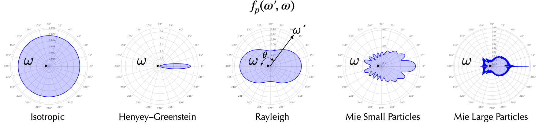
Figure 12.4 visualizes a few common phase functions. While \(f_p(\cdot)\) is technically a 4D function parameterized by \(\os\) and \(\oi\), the phase function of many natural media is 1D and depends only on the angle \(\theta\) subtended by \(\os\) and \(\oi\). In Figure 12.4, the distance of a point on the contour to the center represents the magnitude of the phase function at that particular \(\theta\) Consider under what conditions this simplification can be true:

• First, it says that the phase function does not depend on the absolute incident direction \(\oi\) but the relative angle between \(\oi\) and \(\os\). To get a visual intuition, see Figure 12.5; if the phase function is invariant to the photon incident direction \(\oi\), we can, without losing any generality, assign \(\oi\) to the \(z\)-axis; the scattered direction \(\os\) is parameterized by \(\theta\) and \(\phi\).
• Second, it also says the phase function depends on only \(\theta\) but not \(\phi\). That is, the phase function is rotationally symmetric about the incident direction \(\oi\). So \(f_p(\os, \oi) = f_p(\os', \oi) \neq f_p(\os'', \oi)\).

Figure 12.5: The phase function of a spherical particle is 1) invariant to the incident direction \(\oi\), which, without losing generality, is taken to be the \(z\)-axis here, and 2) also invariant to the azimuthal angle \(\phi\) of the outgoing direction \(\os\) but depends on the polar angle \(\theta\). So \(f_p(\os, \oi) = f_p(\os', \oi) \neq f_p(\os'', \oi)\). Media consisting of such particles are called isotropic media, but it does not mean the particle itself is an isotropic scatterer, which does not exist, but if it did, its phase function would be a constant (invariant to both \(\theta\) and \(\phi\)).

Intuitively, the phase function has the following two properties:

• If you fix the incident direction, no matter how you rotate the particle, the phase function distribution is the same. Alternatively, if you change the incident direction, the phase function distribution moves along with the incident direction.
• Given an incident direction, the phase function distribution is axially symmetric about the incident direction.

The two conditions above are met only when the medium consists of randomly distributed spherically symmetric particles⁴, in which case 1) there is no reason to think that any incident direction is special, so the phase function certainly is invariant to \(\oi\), and 2) there is no reason to think \(\os\) and \(\os'\) are any different since one should not expect the scattering behavior to change if we rotate the sphere about the incident direction (\(z\)-axis).

A medium consisting of spherically symmetric particles is called a symmetric or an isotropic medium. Usually when we refer to an isotropic medium, not only is the phase function but also the total scattering coefficient \(\sigma_s(p, \oi)\) (Equation 12.21) rotationally invariant to the incident direction⁵.

As we said earlier, “isotropic” is an unbelievably overloaded term. People also call a particle an isotropic scatterer if its phase function is a constant, i.e., invariant to \(\os\); such a phase function is sometimes called an isotropic phase function. An isotropic scatterer does not exist; it is a purely theoretical construction, but if it existed, its phase function would take the value of \(\frac{1}{4\pi}\) given Equation 12.18, as shown in the first graph in Figure 12.4.

12.2.4 Common Models and General “Rules”

There are many factors that determine the exact scattering efficiency and scattering direction, which can be calculated by solving the Maxwell’s equations. We will talk about a few common models here; we focus on the intuitions while omitting the exact mathematical expressions, which can be found in standard texts. From the models, we can identify a few general “rules” or, rather, approximations under certain assumptions.

The main theory or model for a single scattering event is called the Mie scattering theory, which, strictly speaking, applies only when the particle is spherical (Sharma 2003, chap. 3.5.2; Bohren and Clothiaux 2006, chap 3.5; Melbourne 2004, chap. 3). Mie scattering is not somehow a different scattering process from any other scattering, and the Mie theory is nothing more than the solution to the Maxwell’s equations under certain conditions⁶.

The Mie theory predicts that the overall scattering efficiency \(Q_s\) is:

\[ \begin{aligned} Q_s &= \frac{8}{3}\gamma^4\big(\frac{m^2-1}{m^2+2}\big)\big[1+\frac{6}{5}\big(\frac{m^2-1}{m^2+2}\big)\gamma^2 + \cdots \big]\\ \gamma &= \frac{r}{\lambda_m}, \\ m &= \frac{n}{n_m}, \end{aligned} \tag{12.22}\]

where \(m\) is the the relative refractive index between the particle and the medium surrounding the particle, and \(\gamma\) is the ratio between the particle radius \(r\) and the incident light wavelength in the surrounding medium \(\lambda_m\). The notion of surrounding media might come across as a little surprising: doesn’t the material consist merely of its particles? Hardly. For instance, in paints, pigments are surrounded by binders (e.g., linseed oil in oil paints, egg yolk in tempera paints, and beeswax in encaustic paints) and usually some amount of water (except oil paints). When paint dries, some water might be evaporated, leaving pockets of air, which also contributes to the surrounding media.

We can draw a few general conclusions from the model.

Small-Particle (Rayleigh) Scattering

For small particles where \(\gamma \ll 1\) (generally when the radius is ten times smaller than the wavelength of the incident light), only the first term in Equation 12.22’s bracket matters, so the scattering efficiency is inversely proportional to \(\lambda_m^{-4}\). The inverse proportionality to \(\lambda_m^{-4}\) largely (but apparently not entirely) explains why the sky is blue and why the sun is red (Bohren and Clothiaux 2006, chap. 8.1). Why? First, recognize that individual molecules, such as air molecules, are usually sub-nm in size, so they scatter in this small-particle regime. Short wavelength lights from the sun are scattered by the atmospheric molecules more toward the sky and eventually enter your eyes, so if you look at the sky (against the sun) it would appear blue; when you look at the sun directly, the photons entering your eyes are mostly those unscattered ones that transmit directly through the atmosphere, and they are mostly longer-wavelength photons.

By then water molecules are also similarly small, so why would water look so different from the air? It is because water molecules are very densely packed, so their scatterings are coherent. In fact, the end result of such coherent scatterings by a collection of water molecules is that water appears specular.

The photopigments in a photoreceptor are very small in size compared to the wavelengths of visible light (each rhodopsin has a cross-section area of about 10^-2 \(\text{nm}^\text{2}\) (Milo and Phillips 2015, p. 144)), so they almost do not scatter lights at all, only absorption. That is why we could use microspectrophotometry (MSP) to measure a photoreceptor’s (transverse) absorption rate (Section 3.2.1): MSP measures the amount of light transmitted through a photoreceptor, and if there is little scattering, then all the photons that are not measured must be absorbed by the photoreceptor.

Scattering in the small-particle regime is also called Rayleigh scattering, which, again, is not somehow a fundamentally different scattering process, and the Rayleigh scattering theory⁷ is nothing more than a special case of the Mie scattering theory (Sharma 2003, chap. 3.5.1; Bohren and Clothiaux 2006. chap. 3.2).

The phase function in the Rayleigh regime is proportional to \(1+\cos^2\theta\), so the backward and forward scatterings are roughly equally probable. Taking the phase function into account, the scattering efficiency (in the form defined in Equation 12.20) in Rayleigh scattering is proportional to:

\[ Q_s \propto (\frac{r}{\lambda_m})^4 \frac{m^2-1}{m^2+2} (1 + \cos^2\theta). \]

Impact of Particle Size

When the particle size increases, the scattering efficiency increases, initially very quickly, but eventually saturates. In fact, the Mie theory predicts that when the particle size is much larger than the wavelength (e.g., more than 100 times larger), the scattering efficiency approaches a constant 2 regardless of \(m\) and \(\lambda_m\) (Johnsen 2012, fig. 5.4). This is evident in Figure 12.6, which shows the scattering efficiency of a kind of particle as a function of particle radius (\(x\)-axis) under different \(m\) (different curves); the incident light wavelength is 500 \(\text{nm}\).

Figure 12.6: Scattering efficiency as a function of particle radius under different relative refractive index \(m\); the incident light wavelength is 500 \(\text{nm}\). From Johnsen (2012, fig. 5.4).

The particle size also affects the phase function. As we have discussed above, small particles in the Rayleigh regime tend to scatter photons equally in the forward and backward directions, while large particles primarily scatter photons in the forward directions. The last two graphs in Figure 12.4 show the phase functions predicted by the Mie scattering theory under different particle sizes (both are larger than that in the Rayleigh regime). The forward fraction increases as the particle size increases.

Consider the scenario in Figure 7.1, where Material₁ sits on top of Material₂, and our goal is to hide Material 2 so that the color of Material 1 is dependent only on the illumination (not the property of Material 2). There is an interesting trade-off between scattering efficiency and scattering direction here. If we want Material 1 to hide Material 2, we want the particles in Material 1 to scatter a lot of light (high scattering efficiency) backwards. If the scattering efficiency is low (so photons march on and are hindered only by absorption) or the scattering is heavy in the forward directions, photons penetrate through Material 1 and reach Material 2, which would then contribute to the overall color.

Now, to scatter a lot of light, we need the particles to be large, but then the scattering will be mostly in the forward directions. So there exists a sweet spot of the particle size that provides the highest “hiding power” for a material per unit volume. If we work out the math, we will see that the sweet spot falls roughly in the visible wavelength range. That is why most paint pigments have a diameter between 100 \(\text{nm}\) and 1 \(\mu\text{m}\) (Bruce MacEvoy 2015). Of course, no matter how poor the hiding power is for a particular paint, if you apply enough of it, it will eventually hide whatever is behind it. Dye pigments are rather small in size (\(\text{nm}\) range), so they scatter few photons and that is why dye solutions look relatively transparent.

Impact of Refractive Index

Figure 12.6 also shows the impact of the relative refractive index \(m\) (between the particle and the surrounding media) on scattering efficiency. Generally, the scattering efficiency increases with \(m\) at all particle sizes until when the particles are so large that the scattering efficiency becomes a constant. This is supported by Equation 12.22, too (\(\frac{m^2-1}{m^2+2}\) monotonically increases and has a limit of 1).

For large particles, while \(m\) does not affect the scattering efficiency, it influences the scattering directions. When \(m\) is small, the scattering tends to be more forward, whereas when \(m\) is large, the scattering tends to be toward large angles (i.e., more photons will be back-scattered). This is why wet objects look darker (recall the unpleasant experience of accidentally spilling water on your pants). In dry paints, the medium surrounding the textile particles is air, and in wet paints it is water. \(m\) becomes smaller when the material is wet (i.e., the relative refractive-index difference becomes smaller between the textile particles and water), so most of the scattering will be forward, increasing the traversal length of photons and essentially giving photons more opportunities to be absorbed.

Aspherical Particles

What if the particle is not spherical? The Mie theory does not apply. Analytical or even numerical solutions to the Maxwell’s equations would be difficult, so perhaps a better approach is just to parameterize a model and fit it with the experimental data.

One popular one-parameter parameterization of the phase function is the Henyey–Greenstein phase function (Pharr, Jakob, and Humphreys 2018, chap. 11.3.1; Bohren and Clothiaux 2006, chap. 6.3.2), which takes the form:

\[ p(\theta) = \frac{1}{4\pi} \frac{1-g^2}{(1+g^2-2g\cos\theta)^{3/2}}, \]

where \(g\) is the free parameter and is usually called the asymmetry parameter.

We hasten to emphasize that the Henyey–Greenstein function has absolutely zero physical meaning; it is designed for fitting experimental phase function data, so in the modern deep learning era, you might as well try a deep neural network. The second graph in Figure 12.4 shows one instantiation of the Henyey–Greenstein function.

Bohren, Craig F, and Eugene E Clothiaux. 2006. Fundamentals of Atmospheric Radiation: An Introduction with 400 Problems. John Wiley & Sons.

Bowmaker, James K, and HJk Dartnall. 1980. “Visual Pigments of Rods and Cones in a Human Retina.” The Journal of Physiology 298 (1): 501–11.

Bruce MacEvoy. 2015. “The material attributes of paints.” https://www.handprint.com/HP/WCL/pigmt3.html#particlesize.

Johnsen, Sönke. 2012. The Optics of Life: A Biologist’s Guide to Light in Nature. Princeton University Press.

Kipp Jones. 2005. “The sand/dust from the harmattan coming from the Sahara gives the Nigeria’s National Mosque in Abuja, a nice glow; CC BY-SA 2.0 license.” https://commons.wikimedia.org/wiki/File:MosqueinAbuja.jpg.

Mayerhöfer, Thomas G, Susanne Pahlow, and Jürgen Popp. 2020. “The Bouguer-Beer-Lambert Law: Shining Light on the Obscure.” ChemPhysChem 21 (18): 2029–46.

Melbourne, William G. 2004. Radio Occultations Using Earth Satellites: A Wave Theory Treatment. 1st ed. John Wiley & Sons.

Milo, Ron, and Rob Phillips. 2015. Cell Biology by the Numbers. Garland Science.

Novák, Jan, Iliyan Georgiev, Johannes Hanika, Jaroslav Křivánek, and Wojciech Jarosz. 2018. “Monte Carlo Methods for Physically Based Volume Rendering.” In ACM SIGGRAPH 2018 Courses.

Pharr, Matt, Wenzel Jakob, and Greg Humphreys. 2018. Physically Based Rendering: From Theory to Implementation. 3rd ed. MIT Press.

Sharma, Gaurav. 2003. “Color Fundamentals for Digital Imaging.” In Digital Color Imaging Handbook, edited by Gaurav Sharma, 14–127. CRC Press.

---

1. “Isotropic” is a very overloaded term; it just means some physical property is invariant when measured from different directions. So depending on what physical property you care about, “isotropic” can mean different things. The property we care about here is a volume’s ability to absorb photons, which is different from our earlier use of isotropy, which is concerned with the ability of a surface to scatter photons.

2. Technically photons from other objects can enter our eye through a single-scattering event; see the discussion at the end.

3. A direction \(\os\) has a solid angle of 0, so its associated irradiance is technically 0, too. What \(f_p(\os, \oi)L(\oi)\doi\) represents is the irradiance per solid angle.

4. or when the medium consists of randomly distributed and oriented spherically asymmetric particles, in which case the medium is statistically spherically symmetric.

5. In theory, it is certainly possible to have a medium whose total scattering coefficient/efficiency varies with the incident direction but not the angular distribution/probability of the scattered photons.

6. The modern form of the solution is summarized, not invented, by Gustav Mie but the solution had been developed by many predecessors such as Ludvig Lorenz.

7. worked out by Lord Rayleigh, who won the Nobel Prize in Physics in 1904