14 Rendering Volume and Subsurface Scattering
\[ \def\oi{{\omega_i}} \def\os{{\omega_s}} \def\Oi{{\Omega_i}} \def\Os{{\Omega_s}} \def\d{{\text{d}}} \def\D{{\Delta}} \def\do{{\d\omega}} \def\Do{{\Delta\omega}} \def\doi{{\d\omega_i}} \def\dos{{\d\omega_s}} \def\Doi{{\D\omega_i}} \def\Dos{{\D\omega_s}} \def\H{{\mathbf{H}}} \newcommand{\cM}{\mathcal{M}} \newcommand{\cL}{\mathcal{L}} \]
So far we have assumed that a ray can only be attenuated, which can happen only when the illumination is collimated and we assume single scattering. Under this assumption, Equation 13.14 allows us to calculate any radiance in the medium (by weakening the initial radiance). General media are much more complicated: illumination can be from anywhere, and multiple scattering must be accounted for. As a result, external photons can be scattered into a ray of interest, as we have intuitively discussed in Section 13.2.1.
In the realm of geometric optics and radiometry, the general way to model lights going through a material/medium amounts to solving the so-called Radiative Transfer Equation (RTE), whose modern version was established by Chandrasekhar (1960)1, and Kajiya and Von Herzen (1984) was the first to introduce it to computer graphics. The RTE provides the mathematical tool to model an arbitrary radiance in a medium (Section 14.1).
We will then discuss an important way to solve the RTE by turning it to the Volume Rendering Equation (VRE) (Section 14.2), discuss the discrete form of the VRE that is commonly used in scientific visualization (Section 14.3) and, more recently, radiance-field rendering (Section 14.4), a modern iteration of image-based rendering (Section 10.2.2) that uses discrete VRE to parameterize the image formation process. Finally, we will show a simple phenomenological model that integrates surface scattering with volume scattering (Section 14.5).
14.1 Radiative Transfer Equation
The basic idea is to set up a differential equation to describe the (rate) of the radiance change. Given an incident radiance \(L(p, \os)\), we are interested in \(L(p+\D s \os, \os)\), the radiance after the ray has gone a small distance \(\D s\). The radiance can be:
- attenuated by the medium because of absorption;
- attenuated by the medium because photons are scattered out into other directions; this is called out-scattering in graphics;
- augmented by photons that are scattered into the ray direction from all other directions — because of multiple scattering2; this is called in-scattering in graphics;
- augmented because particles can emit photons.
The attenuation (reduction) of the radiance over \(\D s\) is:
\[ -L(p, \os) \sigma_t(p, \os) \D s. \tag{14.1}\]
The radiance augmentation due to in-scattering is given by:
\[ \int^{\Omega = 4\pi} f_p(p, \os, \oi) \sigma_s(p, \os) \D s L(\oi) \doi = \sigma_s(p, \os) \D s \int^{\Omega = 4\pi} L(p, \oi) f_p(p, \os, \oi) \doi. \tag{14.2}\]
The way to interpret Equation 14.5 is the following. \(L(p, \oi)\) is the incident radiance from a direction \(\oi\), \(L(p, \oi) \doi\) is the irradiance received from \(\doi\), of which \(\sigma_s(p, \oi)\D s L(p, \os) \doi\) is the irradiance scattered in all directions after traveling a distance \(\D s\). That portion of the scattered irradiance is multiplied by \(f_p(\os, \oi)\) to give us the radiance toward \(\os\) (see Equation 13.19). We then integrate over the entire sphere, accounting for the fact that lights can come from anywhere over the space, to obtain the total augmented radiance toward \(\os\).
If we consider emission, the total radiance augmentation is:
\[ \sigma_a(p, \os) \D s L_e(p, \os) + \sigma_s(p, \os) \D s \int^{\Omega = 4\pi} L(p, \oi) f_p(p, \os, \oi) \doi, \tag{14.3}\]
where \(L_e(p, \os)\) is the emitted radiance at \(p\) toward \(\os\), so the first term represents the total emission over \(\D s\). If we let:
\[ L_s(p, \os) = \sigma_a(p, \os) L_e(p, \os) + \sigma_s(p, \os) \int^{\Omega = 4\pi} L(p, \oi) f_p(p, \os, \oi) \doi, \tag{14.4}\]
the total augmentation can be simplified to:
\[ L_s(p, \os) \D s, \tag{14.5}\]
where the \(L_s\) term is sometimes called the source term or source function in computer graphics, because it is the source of power at \(p\)3.
Combining Equation 14.1 and Equation 14.5, the net radiance change is4:
\[ \begin{aligned} \D L(p, \os) &= L(p + \D s \os, \os) - L(p, \os) \\ &= -L(p, \os) \sigma_t(p, \os) \D s + L_s(p, \os) \D s. \end{aligned} \tag{14.6}\]
As \(\D s\) approaches 0, we get (assuming \(\os\) is a unit vector as in Equation 13.13 and Equation 13.14):
\[ \begin{aligned} \os \cdot \nabla_p L(p, \os) &= \frac{\d L(p, \os)}{\d s} = \lim_{\D s \rightarrow 0} \frac{L(p + \D s \os, \os) - L(p, \os)}{\D s} \nonumber \\ &= -\sigma_t(p, \os) L(p, \os) + L_s(p, \os), \end{aligned} \tag{14.7}\]
where \(\nabla_p\) denotes the gradient of \(L\) with respect to \(p\), and \(\os \cdot \nabla_p\) denotes the directional derivative, which is used because technically \(p\) and \(\os\) are both defined in a three-dimensional space, so what we are really calculating is the rate of radiance change at \(p\) along \(\os\).
Equation 14.7 is the RTE, which is an integro-differential equation, because it is a differential equation with an integral embedded. The RTE has an intuitive interpretation: if we think of radiance as the power of a ray, as a ray propagates, its power is attenuated by the medium but also augmented by “stray photons” from other rays. The latter is given by \(L_s(p, \os)\), which can be thought of as the augmentation of the radiance per unit length.
The RTE describes the rate of change of an arbitrary radiance \(L(p, \os)\). But our ultimate goal is to calculate the radiance itself? Generally the RTE has no analytical solution. There are two strategies to solve it. First, we can derive analytical solutions under certain certain assumptions and simplifications.
For instance, the integral in Equation 14.7 can be approximated by a summation along \(N\) directions; then we can turn Equation 14.7 into a system of \(N\) differential equations to be solved. This is sometimes called the N-flux theory. You might have heard of the famous Kubelka-Munk model (Kubelka and Munk 1931b, 1931a; Kubelka 1948) widely used in modeling the color of pigment mixture; it is essentially a special case of the N-flux theory where \(N=2\), which we will discuss in Section 15.1.
Another assumption people make is to assume that volume scattering is isotropic and can be approximated as a diffusion process. This is called the diffusion approximation (Ishimaru 1977; Ishimaru et al. 1978), which is widely used in both scientific modeling (Farrell, Patterson, and Wilson 1992; Eason et al. 1978; Schweiger et al. 1995; Boas et al. 2001) and in rendering (Stam 1995, chap. 7; Jensen et al. 2001; Dong et al. 2013); see Bohren and Clothiaux (2006, chap. 6.2) for a theoretical treatment.
The second approach deserves its own section.
14.2 Volume Rendering Equation
The second approach, which is particularly popular in computer graphics, is to first turn the RTE into a purely integral equation and then numerically (rather than analytically) estimate the integral using Monte Carlo integration, very similar to how the rendering equation is dealt with for surface scattering (Section 11.3).

The way to think of this is that in order to calculate any given radiance \(L(p, \os)\), we need to integrate all the changes along the direction \(\os\) up until \(p\). Where do we start the integration? We can start anywhere. Figure 14.1 (a) visualizes the integration process. Let’s say we want to start from a point \(p_0\), whose initial radiance toward \(\os\) is \(L_0(p_0, \os)\). Let \(p = p_0 + s\os\), where \(\os\) is a unit vector and \(s\) is the distance between \(p_0\) and \(p\). An arbitrary point \(p'\) between \(p_0\) and \(p\) would then be \(p' = p_0 + s' \os\)5.
Now we need to integrate from \(p_0\) to \(p\) by running \(s'\) from 0 to \(s\). Observe that the RTE is a form of a non-homogeneous linear differential equation, whose solution is firmly established in calculus. Without going through the derivations, its solution is:
\[ L(p, \os) = T(p_0 \rightarrow p)L_0(p_0, \os) + \int_{0}^{s} T(p' \rightarrow p) L_s(p', \os)\d s', \tag{14.8}\]
where \(T(p_0 \rightarrow p)\) is the transmittance between \(p_0\) and \(p\) along \(\os\), and \(T(p' \rightarrow p)\) is the transmittance between \(p'\) and \(p\) along \(\os\). Recall the definition of transmittance in Equation 13.15: it is the remaining fraction of the radiance after attenuation by the medium after traveling the distance between two points. In our case here:
\[ \begin{aligned} T(p' \rightarrow p) = \frac{L(p+s\os, \os)}{L(p+s'\os, \os)} = e^{-\int_{s'}^s \sigma_t(p+t\omega, \omega) \d t}, \\ T(p_0 \rightarrow p) = \frac{L(p+s\os, \os)}{L(p, \os)} = e^{-\int_{0}^s \sigma_t(p+t\omega, \omega) \d t}, \end{aligned} \]
The integral equation Equation 14.8 in the graphics literature is called the volume rendering equation (VRE) or the volumetric light transport equation — the counterpart of the surface LTE (Section 11.3). Looking at the visualization in Figure 14.1 (a), the VRE has an intuitive interpretation: the radiance at \(p\) along \(\os\) is the the contribution of \(p_0\) plus and contribution of every single point between \(p_0\) and \(p\).
- The contribution of \(p_0\) is given by its initial radiance \(L_0\) weakened by the transmittance between \(p_0\) and \(p\);
- Why would a point \(p'\) between \(p_0\) and \(p\) make any contribution? It is because of the source term (Equation 14.4): \(p'\) might emit lights, and some of the in-scattered photons at \(p'\) will be scattered toward \(\os\). The contribution of \(p'\) is thus given by the source term \(L_s\) weakened by the transmittance between \(p'\) and \(p\).
The form of the VRE might appear to suggest that it is enough to accumulate along only the direct path between \(p_0\) and \(p\), which is surprising given that there are infinitely many scattering paths between \(p_0\) and \(p\) (due to multiple scattering). For instance, it appears that we consider only the outgoing radiance toward \(\os\) from \(p_0\), but \(p_0\) might have outgoing radiances over other directions, which might eventually contribute to \(L(p, \os)\) through multiple scattering. Are we ignoring them?
The answer is that the VRE implicitly accounts for all the potential paths between \(p_0\) and \(p\) because of the \(L_s\) term, which expands to Equation 14.4. That is, every time we accumulate the contribution of a point between \(p_0\) and \(p\), we have to consider the in-scattering from all the directions at that point. Another way to interpret this is to observe that the radiance term \(L\) appears on both sides of the equation. Therefore, the VRE must be solved recursively by evaluating it everywhere in space.
Does this remind you of the rendering equation (Equation 11.18)? Indeed, the VRE can be thought of as the volumetric counterpart of the rendering equation. Similarly, we can use Monte Carlo integration to estimate it, just like how the rendering equation is dealt with — with an extra complication: the VRE has two integrals: the outer integral runs from \(p_0\) to \(p\) and, for any intermediate point \(p'\), there is an inner integral that runs from \(p'\) to \(p\) to evaluate the transmittance \(T(p' \rightarrow p)\). Therefore, we have to sample both integrands.
Similar to the situation of the rendering equation, sampling recursively would exponentially increase the number of rays to be tracked. Put it another way, since there are infinitely many paths from which a ray gains its energy due to multiple scattering, we have to integrate infinitely many paths. Again, a common solution is path tracing, for which Pharr, Jakob, and Humphreys (2023, chap. 14) is a great reference.
A simplification that is commonly used is to assume that there is only single scattering directly from the light source. In this way, the \(L_s\) term does not have to integrate infinitely many incident rays over the sphere but only a fixed amount of rays emitted from the light source non-recursively. This strategy is sometimes called local illumination in volume rendering, as opposed to global illumination, where one needs to consider all the possible paths of light transport. The distinction is similar to that in modeling surface scattering (Section 11.3).
14.3 Discrete VRE and Scientific Volume Visualization
Sometimes the VRE takes the following discrete form:
\[ L = \sum_{i=0}^{N-1}\big(L_i\D s\prod_{j=i+1}^{N-1}t_j\big). \tag{14.9}\]
Equation 14.9 is the discrete version of Equation 14.8: the former turns the two integrals in the latter (both the outer integral and the inner one carried by \(T(\cdot)\)) to discrete summations using the Riemann sum over \(N\) discrete points along the ray between \(p_0\) and \(p\) at an interval of \(\D s = \frac{s}{N}\).
The notations are slightly different; Figure 14.1 (b) visualizes how this discrete VRE is expressed with the new notations.
- \(L\) is \(L(p, \os)\), the quantity to be calculated;
- \(L_i\) is a shorthand for \(L_s(p_i, \os)\), i.e., the source term (Equation 14.4) for the \(i^{th}\) point between \(p_0\) and \(p\) toward \(\os\); by definition, \(p_0\) is the \(0^{th}\) point (so \(L_0\) is the initial radiance \(L_0(p_0, \os)\) in Equation 14.8) and \(p\) is the \(N^{th}\) point;
- \(t_i\) (or more explicitly \(t(p_{i} \rightarrow p_{i+1})\)) represents the total transmittance between the \(i^{th}\) and the \((i+1)^{th}\) point and is given by \(e^{-\sigma_t(p_i, \os) \D s}\) (notice the integral in continuous transmittance Equation 13.15 is gone, because we assume the transmittance between two adjacent points is a constant in the Reimann sum);
- \(\alpha_i\) is the opacity between the \(i^{th}\) and the \((i+1)^{th}\) point, which is defined as the residual of the transmittance between the two points: \(1-t_i\).
See Max (1995, Sect. 4) or Kaufman and Mueller (2003, Sect. 6.1) for a relatively straightforward derivation of Equation 14.9, but hopefully this form of the VRE is equally intuitive to interpret from Figure 14.1 (b). It is nothing more than accumulating the contribution of each point6 along the ray, but now we also need to accumulate the attenuation along the way just because of how opacity is defined by convention (per step), hence the product of a sequence of the opacity residuals.
We can also re-express Equation 14.9 using opacity rather than transmittance: \[ \begin{aligned} L &= \sum_{i=0}^{N-1}\big(L_i\D s\prod_{j=i+1}^{N-1}(1-\alpha_j)\big) \\ &= L_{N-1} \D s + L_{N-2} \D s(1-\alpha_{N-1}) + L_{N-3} \D s(1-\alpha_{N-1})(1-\alpha_{N-2}) +~\cdots~ \\ &~~~+ L_1\D s\prod_{j=2}^{N-1}(1-\alpha_j)+ L_0\D s\prod_{j=1}^{N-1}(1-\alpha_j). \end{aligned} \tag{14.10}\]
The discrete VRE is usually used in the scientific visualization literature, where people are interested in visualizing data obtained from, e.g., computer tomography (CT) scans or magnetic resonance imaging (MRI). There, it is the relative color that people usually care about, not the physical quantity such as the radiance, so people sometimes lump \(L_i\D s\) together as \(C_i\) and call it the “color” of the \(i^{th}\) point. The VRE is then written as:
\[ C = \sum_{i=0}^{N-1}\big(C_i\prod_{j=i+1}^{N-1}(1-\alpha_j)\big). \tag{14.11}\]
The \(C\) terms are defined in a three-dimensional RGB space, and Equation 14.11 is evaluated for the three channels separately, similar to how Equation 14.9 and Equation 14.8 are meant to be evaluated for each wavelength independently. Since color is a linear projection from the spectral radiance, the so-calculated \(C\) (all three channels) is indeed proportional to the true color, although in visualization one usually does not care about the true colors anyway (see Section 14.3.3).
Equation 14.11 is also called the back-to-front compositing formula in volume rendering, since it starts from \(p_0\), the farthest point on the ray to \(p\). We can easily turn the order around to start from \(p\) and end at \(p_0\) in a front-to-back fashion (\(C_{N-1}\) now corresponds to \(p_0\)):
\[ C = \sum_{i=0}^{N-1}\big(C_i\prod_{j=0}^{i-1}t_j\big). \tag{14.12}\]
While theoretically equivalent, the latter is better in practice because it allows us to opportunistically terminate the integration early when, for instance, the accumulated opacity is high enough (transmittance is low enough), at which point integrating further makes little numerical contribution to the result.
14.3.1 Another Discrete Form of VRE
A perhaps more common way to express the discrete VRE is to approximate the transmittance \(t\) using the first two terms of its Taylor series expansion and further assume that the medium has a low albedo, i.e., \(\sigma_t \approx \sigma_a\) and \(\sigma_s \approx 0\) (that is, the medium emits and absorbs only); we have:
\[ \begin{aligned} & 1 - \alpha_i = t_i = t(p_{i} \rightarrow p_{i+1}) = e^{-\sigma_t(p_i, \os) \D s} = 1 - \sigma_t(p_i, \os) \D s + \frac{(\sigma_t(p_i, \os) \D s)^2}{2} - \cdots \\ \approx & 1 - \sigma_t(p_i, \os) \D s \\ \approx & 1 - \sigma_a(p_i, \os) \D s. \end{aligned} \]
Therefore:
\[ \alpha_i \approx \sigma_a(p_i, \os) \D s. \tag{14.13}\]
Now, observe that the \(L_i\) term in Equation 14.9 is the source term in Equation 14.4, which under the low albedo assumption has only the emission term, so:
\[ \begin{aligned} L &= \sum_{i=0}^{N-1}\big(L_i\D s\prod_{j=i+1}^{N-1}(1-\alpha_j)\big) \\ &= \sum_{i=0}^{N-1}\big(\sigma_a(p_i, \os) L_e(p_i, \os)\D s\prod_{j=i+1}^{N-1}(1-\alpha_j)\big). \end{aligned} \tag{14.14}\]
Now plug in Equation 14.13, we have:
\[ L = \sum_{i=0}^{N-1}\big(L_e(p_i, \os)\alpha_i\prod_{j=i+1}^{N-1}(1-\alpha_j)\big). \tag{14.15}\]
If we let \(C_i = L_e(p_i, \os)\), the discrete VRE is then expressed as (Levoy 1988):
\[ C = \sum_{i=0}^{N-1}\big(C_i\alpha_i\prod_{j=i+1}^{N-1}(1-\alpha_j)\big). \tag{14.16}\]
This can be interpreted as a form of alpha blending (Smith 1995), a typical trick in graphics to render transparent materials. It makes sense for our discrete VRE to reduce to alpha blending: our derivation assumes that the volume does not scatter lights, so translucent materials become transparent.
Again, Equation 14.16 is the back-to-front equation, and the front-to-back counterpart looks like:
\[ C = \sum_{i=0}^{N-1}\big(C_i\alpha_i\prod_{j=0}^{i-1}t_j\big). \tag{14.17}\]
If you compare the two discrete forms in Equation 14.11 and Equation 14.16, it would appear that the two are not mutually consistent! Of course we know why: 1) Equation 14.16 applies two further approximations (low albedo and Taylor series expansion) and 2) the two \(C\) terms in the two equations refer to different physical quantities (compare Equation 14.10 with Equation 14.15).
14.3.2 The Second Form is More Flexible
What is the benefit of this new discrete form, comparing Equation 14.12 and Equation 14.17? Both equations can be interpreted as a form of weighted sum, where \(C_i\) is weighted by a weight \(w_i\), which is \(\prod_{j=0}^{i-1}t_j\) in the first case and \(\alpha_i\prod_{j=0}^{i-1}t_j\) in the second case. The most obvious difference is that the weights in the first case are correlated but less so in the second case: the weights are strictly decreasing as \(i\) increases in the first case, since \(t_i < 1\).
In the second case, the weights are technically independent. Observe, in the second case, that \(w_0 = \alpha_0\) and \(w_{i+1} = w_i \frac{\alpha_{i+1}(1-\alpha_i)}{\alpha_i}\), so there is generally a unique assignment of the \(\alpha\) values for a given weight combination. This “flexibility” will come in handy when we can manually assign (Section 14.3.3) or learn the weights (Section 14.4). Note, however, that if we impose the constraint that \(\alpha\in[0, 1]\), we are effectively constraining the weights in the second case, too.
14.3.3 Visualization is Not (Necessarily) Physically-Based Rendering!
These discrete VRE forms might give you the false impression that we have avoided the need to integrate infinitely many paths, because, computationally, the evaluation of the VRE comes down to a single-path summation along the ray trajectory. Not really. Calculating the \(C_i\) terms in the new formulations still requires recursion if the results are meant to be physically accurate. Of course we can sidestep this by, e.g., applying the local-illumination approximation, as mentioned before, to avoid recursion.
Scientific visualization offers another opportunity: we can simply assign values to the \(C\)s and even the \(\alpha\)s without regard to physics. The goal of visualization is to discover/highlight interesting objects and structures while de-emphasizing things that are irrelevant. So the actual colors are not as important, which gives us great latitude to determine VRE parameters.

Figure 14.2 compares volume-rendered images for scientific visualization (a) and for photorealistic rendering (b). In the case of visualization, the data were from CT scans. In both scans, the outer surface is not transparent but is rendered so just because we are interested in seeing the inner structures that are otherwise occluded. The user makes an executive call to assign a very low transparency to the bones in the knee model 0 but a very high transparency value to the skin and other tissues: this is not physically accurate but a good choice for this particular visualization. Photorealistic rendering, in contrast, has to be physically based and does not usually have this flexibility. See figures in Wrenninge and Bin Zafar (2011) and Fong et al. (2017) for more examples.
There is volume rendering software that would allow the users to make such an assignment depending on what the user wants to highlight and visualize. With certain constraints and heuristics, one can also procedurally assign the \(\alpha\) and \(C\) values from the raw measurement data, usually a density field (see below) acquired from whatever measurement device is used (e.g., CT scanners or MRI machines), using what is called the transfer functions in the literature7. Making an assignment usually is tied to a classification problem: voxels/points of different classes should have different assignments.
14.3.4 Density Fields
Physically speaking, the medium in RTE/VRE is parameterized by its absorption and scattering coefficients, which are a product of cross section and concentration, which is sometimes also called the density. In physically-based volume rendering, this is indeed how the density is used from the very beginning (Kajiya and Von Herzen 1984; Blinn 1982).
In visualization where being physically accurate or photorealistic is unimportant, the notion of an attenuation coefficient8 loses its physical meaning; it is just a number that controls how the brightness of a point weakens. People simply call the attenuation coefficient the density (Kaufman and Mueller 2003), presumably because, intuitively, if the particle density is high the color should be dimmer. If you want to be pedantic, you might say that the attenuation coefficient depends not only on the density/concentration but also on the cross section (Equation 13.2), so how can we do that? Remember in visualization one gets to make an executive call and assign the density value (and thus control \(\alpha\)), so it does not really matter if the value itself means the physical quantity of density/concentration. This is apparent in early work that uses volume rendering for scientific visualization (Sabella 1988; Williams and Max 1992), where attenuation coefficients are nowhere to be found.
For this reason, the raw volume data obtained from raw measurement device for scientific (medical) visualization are most often called the density field, even though what is being measured is almost certainly not the density field but a field of optical properties that are related to, but certainly do not equate, density. For instance, the raw data you get from a CT scanner is actually a grid of attenuation coefficients (Bharath 2009, chap. 3).
14.4 Discrete VRE in (Neural) Radiance-Field Rendering
There is another field where the discrete VRE (especially our second form Equation 14.16) is becoming incredibly popular: (neural) radiance-field rendering. The two most representative examples are NeRF (Mildenhall et al. 2021) and 3D Gaussian Splatting (3DGS) (Kerbl et al. 2023). They are fundamentally image-based rendering or light-field rendering (Section 10.2), where they sample the light field of the scene by taking a set of images at different camera poses and learn to reconstruct the underlying light field, from which they can then re-sample a new camera pose and, thus, render the corresponding image as if it was taken at that new camera pose. This is re-branded in the modern era as “novel view synthesis”.
We will assume that you have read the two papers above so that we can focus on interpreting these radiance-field methods within the fundamental framework of physically-based rendering. Such a re-interpretation would allow us to better understand where these methods come from, how they have introduced new tweaks to physically-based rendering, and what their limitations might be.
The first thing to notice is that NeRF and 3DGS, being essentially a sampling and reconstruction method, use the discrete form of the VRE (mostly Equation 14.16) as the reconstruction function. This means they assume that the radiance is calculated by a single-path summation along the ray trajectory without the need for path tracing and solving the actual RTE/VRE. The reason they can reduce infinite paths to a single-path evaluation is very similar to that in scientific visualization, except now instead of assigning the “color” values \(C\) and opacity values \(\alpha\) (or equivalently the density field as discussed above), they train a neural network to directly learn these values.
14.4.1 VRE for Surface Rendering?
It is interesting to observe that both NeRF and 3DGS (and the vast majority of their later developments) use the discrete VRE form in Equation 14.16 as their forward model and can evidently do a very good job at rendering opaque surfaces. Is this surprising? Isn’t Equation 14.16 designed to render transparent materials/volumes (alpha blending)?
For opaque surfaces, the “ground truth” is the surface rendering equation (Section 11.3), which can be seen as a form of weighted sum, where the BRDF \(f_r(p, \os, \oi)\) weighs the incident light irradiance \(L(p, \oi) \cos\theta_i \text{d}\oi\). In theory, the weights are independent of each other: the value of \(f_r(p, \os, \oi)\) at different \(\oi\) can technically be completely uncorrelated. But in reality they are most likely somewhat correlated for real materials: the appearance of a material does not change dramatically when the incident light direction changes slightly. For volumes/translucent materials, the “ground truth” is the VRE, which you could also say is a weighted sum, although the weights are constrained if the \(\alpha\) values are constrained (e.g., between 0 and 1), which is the case in NeRF and 3DGS training (Section 14.3.2).
So effectively, when rendering opaque surfaces, we are using a form of (theoretically) constrained weighted sum to approximate another (practically) constrained weighted sum, and we hope that we can learn the approximation from a large amount of offline samples. The learned parameters (color and opacity of each point) should not be interpreted literally in the physical sense. One advantage of this parameterization is that it could be used to render volumes or translucent materials if needed, where the ground truth is the VRE, in which case the learned parameters might be more amenable to physical interpretations.
14.4.2 Volume Graphics vs. Point-Based Graphics
Related to volume graphics, there is also a subtly different branch of graphics called point-based graphics (PBG) (Levoy and Whitted 1985; Gross and Pfister 2011). The boundary is somewhat blurred, but given the way the two terms are usually used, we can observe a few similarities and distinctions. Both volume graphics and PBG use discrete points as the rendering primitives (as opposed to continuous surfaces such as a mesh), although the input points in volume graphics are usually placed on uniform grids (Engel et al. 2006, chap. 1.5.2) whereas points in PBG can be spatially arbitrary.
Traditionally, PBG is almost exclusively used for photorealistic rendering of surfaces. In fact, the points used in PBG are usually acquired as samples on continuous surfaces (Gross and Pfister 2011, chap. 3). PBG usually uses object-order rendering through splatting, although ray casting is used too, but RTE/VRE is not involved in the rendering process (Gross and Pfister 2011, chap. 6).
In contrast, the use of volume graphics is much broader. Volume rendering can be used for photorealistic rendering of participating media and translucent surfaces (by solving the RTE/VRE), or it can be used for non-photorealistic data visualization (by evaluating the single-path, discrete VRE), at which point whether the object to be rendered is called a participating medium, a translucent surface, or anything else is irrelevant, because visualization does not care much about being physically accurate.
3DGS is a somewhat interesting case. It is largely a form of PBG because the rendering primitives are unaligned surface samples, and its splatting technique (which we will discuss shortly) resembles that developed in the PBG literature (Gross and Pfister 2011, chap. 6.1). However, 3DGS does use the discrete VRE as the forward model. Again, as discussed just above, VRE is just a way for 3DGS to parameterize its forward mode, so the comparison with traditional volume graphics and PBG should not be taken literally.
14.4.3 Splatting is Signal Filtering
Splatting, initially proposed by Westover (1990) for visualizing volume data, is a common rendering technique used in PBG and 3DGS-family models. We discuss what splatting is, why it works, and how it is used in NeRF and 3DGS. We start by asking: how can we render continuous surfaces from discrete points? If we directly project the points to the sensor plane, we obviously will get holes, as shown in Figure 14.3 (a). This is, of course, not an issue if the rendering primitives are meshes (or procedurally-generated surfaces).
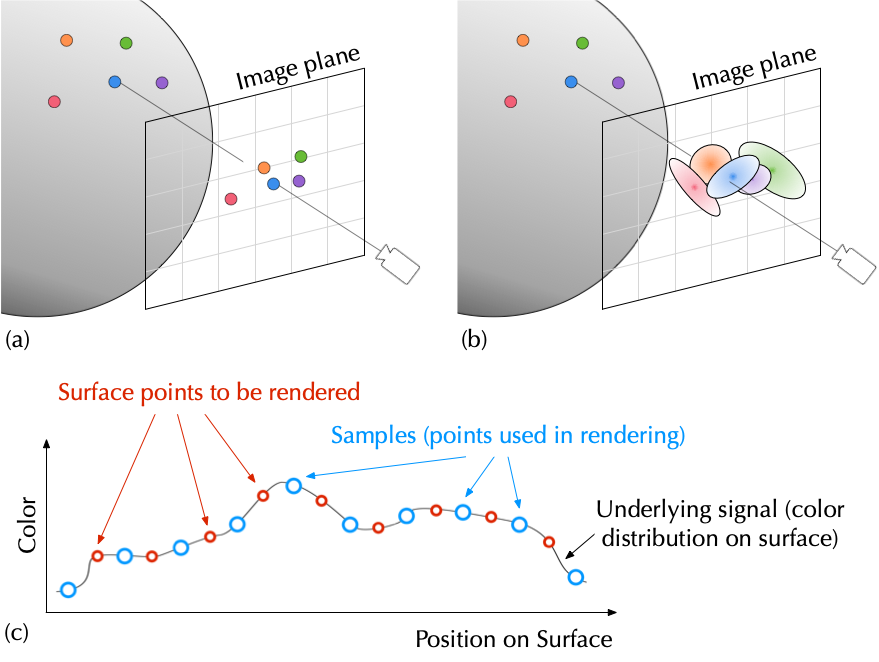
The key is to realize that “meshless” does not mean surfaceless: the fact that we do not have a mesh as the rendering primitives does not mean the surface does not exist. Recall that the points used by PBG are actually samples on the surface. To render an image pixel is essentially to estimate the color of a surface point that projects to the pixel (ignoring supersampling for now). From a signal processing perspective, this is a classic problem of signal filtering: reconstruction and resampling.
That is, ideally what we need to do is to reconstruct the underlying signal, i.e., the color distribution of the continuous surface9 (combined with an anti-aliasing pre-filter10) and then resample the reconstructed/filtered signal at positions corresponding to pixels in an image. This is shown in Figure 14.3 (c). %This amounts to applying a single composite filter \(F\) at new sampling positions, and The name of the game is to design proper filters. The issue of signal sampling, reconstruction, and resampling is absolutely fundamental to all forms of photorealistic rendering and not limited to PBG; Pharr, Jakob, and Humphreys (2023, chap. 8) and Glassner (1995, Unit II) are great references.
Another way to think of this is that the color of a surface point is very likely related to its nearby points that have been sampled as part of the rendering input, so one straightforward thing to do is to interpolate from those samples to calculate colors of new surface points. Signal interpolation is essentially signal filtering/convolution.
There is one catch. In classic signal sampling theories (think of the Nyquist-Shannon sampling theorem), samples are uniformly taken and, as a result, we can use a single reconstruction filter. But in PBG the surface samples are non-uniformly taken, so a single reconstruction filter would not work. Instead, we need a different filter for each point. The filter in the PBG parlance is called a splat, or a footprint function; it is associated with each point (surface sample) and essentially distributes the point color to a local region, enabling signal interpolation. This is shown in Figure 14.3 (b). The exact forms of the footprint functions would determine the exact forms of the signal filters. Gaussian filters are particularly common, and Gaussian splatting is a splatting method that uses Gaussian filters (Greene and Heckbert 1986; Heckbert 1989; Zwicker et al. 2001b).
From a 3D modeling perspective, instead of having a continuous mesh, the scene is now represented by a set of discrete points, each of which is represented by a 2D Gaussian distribution, which is called a surface element or a surfel (Pfister et al. 2000). Each surfel is then projected to the screen space to generate a splat as the corresponding reconstruction kernel of that surface point; the reconstruction kernel, after projection, is another Gaussian filter (which can be cascaded with an anti-aliasing pre-filter). The color of each screen space point is then calculated by summing over all the splats (each of which is, of course, scaled by the color of the sample), essentially taking a weighted sum of the colors of the neighboring surface samples (see Zwicker et al. (2001b, fig. 3) for a visualization) or, in signal processing parlance, resampling the reconstructed signal with the reconstruction kernels.
This rendering process is traditionally called surface splatting (Zwicker et al. 2001b). Yifan et al. (2019) is an early attempt to learn the surfels through a differential surface splatting process. Surface splatting is a reasonable rendering model in PBG: the “ground truth” in rendering surfaces is the rendering equation, which can also be interpreted as a weighted sum.
One can also apply the same splatting idea to volume rendering. In this case, each point in the scene is represented by a 3D Gaussian distribution, which is projected to a 2D splat in the screen space. The color of a pixel is then calculated through, critically, alpha blending the corresponding splats, not weighted sum. This is called volume splatting (Zwicker et al. 2001a). 3DGS can be seen as a differential variant of traditional volume splatting, even though it is also very effective in rendering opaque surfaces (and we have discussed the reason on Section 14.4.1).
14.5 Integrating Surface Scattering with Volume Scattering
The rendering equation governs the surface scattering or light transport in space, and the RTE/VRE governs the volume/subsurface scattering or light transport in a medium. Both processes can be involved in a real-life scene. For instance, the appearance of a translucent material like a paint or a wax is a combination of both forms of scattering/light transport (Figure 8.1). Another example would be rendering smoke against a wall.
Conceptually nothing new needs to be introduced to deal with the two forms of light transport together. Say we have an opaque surface (a wall) located with a volume (smoke) in the scene. If we want to calculate the radiance of a ray leaving a point on the wall, we would evaluate the rendering equation there, and for each incident ray, we might have to evaluate the VRE since that ray might come from the volume. In practice it amounts to extending the path tracing algorithm to account for the fact that a path might go through a volume and bounce off between surface points. See Pharr, Jakob, and Humphreys (2023, chap. 14.2) and Fong et al. (2017, Sect. 3) for detailed discussions.
Another approach, which is perhaps more common when dealing with translucent materials (whose appearance, of course, depends on both the surface and subsurface scattering), is through a phenomenological model based on the notion of Bidirectional Scattering Surface Reflectance Distribution Function (BSSRDF) (Nicodemus et al. 1977). The BSSRDF is parameterized as \(f_s(p_s, \os, p_i, \oi)\), describing the infinitesimal outgoing radiance at \(p_s\) toward \(\os\) given the infinitesimal power incident on \(p_i\) from the direction \(\oi\):
\[ f_s(p_s, \os, p_i, \oi) = \frac{\text{d}L(p_s, \os)}{\text{d}\Phi(p_i, \oi)}. \tag{14.18}\]
BSSRDF can be seen as an extension of BRDF in that it considers the possibility that the radiance of a ray leaving \(p_s\) could be influenced by a ray incident on another point \(p_i\) due to SSS/volume scattering. Given the BSSRDF, the rendering equation can be generalized to:
\[ L(p_o, \os) = \int^A\int^{\Omega=2\pi} f_s(p_s, \os, p_i, \oi) L(p_i, \oi) \cos\theta_i \doi \d A, \tag{14.19}\]
where \(L(p_o, \os)\) is the outgoing radiance at \(p_o\) toward \(\os\), \(L(p_i, \oi)\) is the incident radiance at \(p_i\) from \(\oi\), \(A\) in the outer integral is the surface area that is under illumination, and \(\Omega=2\pi\) means that each surface point receives illumination from the entire hemisphere.
We can again use path tracing and Monte Carlo integration to evaluate Equation 14.19 if we know the BSSRDF, which can, again, either be analytically derived given certain constraints and assumptions or measured (Frisvad et al. 2020). To analytically derive it, one has to consider the fact that the transfer of energy from an incident ray to an outgoing ray is the consequence of a cascade of three factors: two surface scattering (refraction) factors, one entering the material surface \(p_i\) from \(\oi\) and the other leaving the material surface at \(p_i\) toward \(p_o\), and a volume scattering factor that accounts for the subsurface scattering between the incident ray at \(p_i\) and the exiting ray at \(p_o\) (Pharr, Jakob, and Humphreys 2018, chap. 11.4). If all three factors have an analytical form, the final BSSRDF has an analytical form too. This is the approach that, for instance, Jensen et al. (2001) takes.
Subrahmanyan Chandrasekhar won the Nobel Prize in physics in 1983 (not for the RTE).↩︎
Technically, even single scattering can lead to augmentation if there is illumination coming from anywhere outside the ray direction.↩︎
Some definitions do not include emission in the source term, while in other definitions the source term is what is defined here divided by \(\sigma_t\).↩︎
A subtlety you might have noticed is that not all the out-scattering of \(L(p, \os)\) attenuates the radiance; some of the scattering could be toward \(\os\) so should augment the radiance. This is not a concern since our augmentation term Equation 14.5 integrates over the entire sphere, so it considers \(L(p, \os)\) again as part of in-scattering and accounts for the forward-scattered portion of \(L(p, \os)\).↩︎
There are two alternative parameterizations, both of which are common in graphics literature. The first (Pharr, Jakob, and Humphreys 2023) is to express \(p_0 = p + s\os\) (\(s\) being positive), but then the initial radiance would have to be expressed as \(L(p_0, -\os)\), since \(\os\) now points from \(p\) to \(p_0\). The other is to express \(p_0 = p - s\os\) (\(s\) again being positive) (Fong et al. 2017); this avoids the need to switch directions but uses a negative sign. It is a matter of taste which one to use, but be alert to the different conventions.↩︎
technically it is the contribution of each small segment between two discrete points because of the Reimann sum.↩︎
Some (color) transfer functions could have physical underpinnings, such as applying a single-scattering shading algorithms (i.e., local illumination); see, e.g., Levoy (1988, Sect. 3) or Max (1995, Sect. 5), but the goal there is not to precisely model physics but for better, subjective visualization.↩︎
which is the only coefficient needed and which participates in calculating \(\alpha\) (Equation 14.11).↩︎
assuming a diffuse surface so we care to reconstruct the color of each point, not the radiance of each ray.↩︎
The compound filter combining reconstruction and anti-aliasing filters is sometimes also called a resampling filter, because the compound filter is used during resampling to calculate the new sample values.↩︎